Activities Using Bad Elf GPS

Introduction
The purpose of this activity was to become more familiar with the Bad Elf GPS unit by pairing it with a cell phone application and mapping an area on the UW - Eau Claire campus.  The class was split into groups and set off to walk paths/patterns of choice.  Line features were tracked using the Bad Elf, the paths were stored in the iphone app, and maps were to be created from the results.

This activity also had the purpose of exposing students to some other possible cell phone applications that are useful in collecting data and storing them within a cell phone.  These apps include: Collector, Survey 123, GIS4 Mobile, Theodolite, GAIA GPS, and Galileo Offline Maps.  Some of these were to be used later in the class and some others could be useful tools in other projects or recreational activities.  The use of survey GPS units that can pair with cell phones through Bluetooth is becoming increasingly popular because it is cheaper to use cell phone apps than to create a large screen on the same GPS device with the same level of functionality. 

Study Area
The study area was UW - Eau Claire's lower campus, as shown in Figure 1.

Figure 1: The map of UW - Eau Claire's lower campus within the city of Eau Claire.

Methods
The first step was to download the Bad Elf App to the iphone.  Next the Bad Elf was used to record a tracklog of the path walked, which could later be exported as a KML or a GPX file by pairing with the cell phone.  Then a logfile was started, and line features were recorded by walking around various sections of lower campus.  Once those were completed the tracklog was uploaded to the phone. Within the phone app then it was shared as a KML in an email to each group member.   This KML was used to create a map in ArcGIS Earth that shows the tracklog from the activity, as seen in the results.


Results

Figure 2: The tracklog is shown in this map in ArcGIS Earth.  

The map in Figure 2 shows the tracklog taken with the Bad Elf GPS.  It is zoomed out quite far because zooming in closer showed imagery that was not up to date where the path would be crossing through old buildings on campus.  Though this result doesn't quite show high accuracy or direction, it is a good example of a quick tracklog that can be taken and uploaded to ArcGIS Earth. 


Conclusion
This activity gave a chance to work with a basic GPS device that can be paired with a cell phone through Bluetooth to connect to an application where the tracklog can be exported to any destination.  It was a simple method for acquiring a fairly accurate path. 

Creation of Navigation Maps

Introducion/Background
This purpose of this activity was to create two navigation maps.  They will later be used for actual navigation in a field activity.  Map elements that would be helpful with navigation were to be included in the final maps.

Study Area
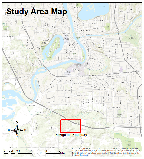
The area in which we will map and navigate is the Priory, just South of Eau Claire. Figure 1 shows the study area.

Figure 1: The study area map with the Navigation Boundary in red.

Methods
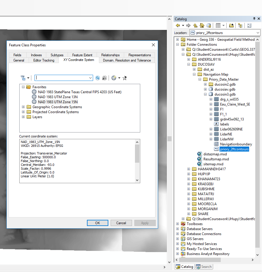
Map data was provided by Professor Hupy, but all layers were in different projections.  The projections were then each defined in ArcCatalog to be Transverse_Mercator with  NAD_1983_UTM_Zone_15N as the coordinate system, since Eau Claire falls within UTM Zone 15.  This is shown in Figure 2.

Figure 2: Each feature is assigned the same coordinate system so they are in the correct place when brought into the map.  

Each student was then able to choose which layers to include in their navigation maps.  I decided to use the imagery basemap from ArcGIS as the background for my map so that specific features could be easily identified, as shown in Figure 3.

Figure 3: This is the defined area's boundary and the imagery basemap.  

The next step was to include a grid in the map.  Grids can be created in the Layers Properties.  Figure 4 shows some of the properties of the grid created for this map.  Each interval is set at 50 meters, which is a reasonable distance for navigation on foot.

Figure 4: This shows some properties of the grid created for this map.  

A new map was then made with the same data and projection but a different grid.  This grid was made in decimal degrees.  Figure 5 shows some properties of this new grid.  The intervals are set at 5".

Figure 5: This grid is for the decimal degrees navigation map.  

Results 

Figure 6: The final UTM navigation map.  

Figure 6 shows the final UTM navigation map.  This could be used for locating landmarks shown in the imagery basemap.  It has a tighter grid than the decimal degrees map, so it could be useful for finding a more exact location.  

Figure 7: The final decimal degrees navigation map.  

Figure 7 shows the final decimal degrees navigation map.  It has slightly larger grid areas that are rectangular, and could be useful as a map for a general area that is not quite as specific as the other map.  It slits the area into larger areas, but can also utilize the imagery in the map to locate land features. 

Conclusion
There are several ways a navigation map can be created and displayed.  The final product should be functional and should pertain to the intended use of the navigation activity.  The final map results from this activity demonstrate only a couple variations of elements that could be included in this type of map.  Other things like contour lines, hillshade, etc. could help show the terrain and slope of the landscape better, or other types of basemaps could show characteristics of the land that may not be captured in the imagery basemap. 

Litchfield Mine Field Surveying Activities

Introduction
On Saturday, September 30th the class visited the Litchfield Mine to make an evaluation of UAS platforms and GPS units for ground control.  Some of the main goals of this trip were to: personally lay ground control points (GCP's), observe the difference in consumer grade and survey grade GPS devices, and weigh the pros and cons between different types of unmanned aerial system (UAS) platforms.  The data collected will be later processed and analyzed, so detailed note taking throughout the day was important.

The Litchfield Mine is an aggregate mine that contains large piles of different rock, sand, and other material.  This mine is regularly surveyed to determine how much material has been deposited or taken from the piles.  Unmanned aerial systems (drones) can be used as a method of surveying the mine to measure the sizes of each pile of material.  This is done by laying ground control points and noting the exact location of each using GPS.  The imagery taken throughout the flight path of the drone is then brought into a GIS and the imagery is laid down onto a map by pinpointing the exact location of each of those GCP's.  This is also known as georeferencing.  This is a relatively new form of technology so the entire surveying industry does not rely on UAS, but this emerging surveying method shows promising efficiency.

UAS professionals from the surveying industry were invited by Professor Joseph Hupy to give demonstrations using their survey grade UAS platforms and other surveying technology.  Professionals from Topcon Solutions and Menet Aero came to work with us in the field.  They provided some cutting edge drones as well as a wealth of knowledge about the industry and new technology.

The study area is shown in Figure 1.

Figure 1: This map shows the location of the Litchfield Mine, near Eau Claire, Wisconsin.  

Methods
The first step we took in surveying the mine was laying down ground control points.  The class laid 16 GCP's throughout the mine.  Each GCP is about a 2' x 2' colored square marker with a center point from which to measure the exact GPS location.  The more GCP's used in a survey the more accurate the survey can be when it is georeferenced later.  They must also be spread wisely throughout the mine.  If some GCP's are too bunched together it can create warping of the imagery when being georeferenced.  The location of all the GCP's were noted in a rough drawing in a field notebook so that none of them were lost in the process.

Once all the GCP's were set we measured the GPS location using three different devices: the Topcon HiPer, the Bad Elf GPS, and an iphone.  This is shown in Figure 2.  The Bad Elf and iphone locations were recorded by the students, and the Topcon HiPer units were recorded by the professionals. The professionals from Menet Aero also laid down Arrow GPS markers to make some extra GCP's, as seen in Figure 3.  Each marker is solar powered and waterproof, and they record their GPS location with the press of a button.

Figure 2: This picture shows GCP #8.  Peter from Menet Aero records the location with the Trimble R2, while my group members record the locations from the Bad Elf and the iphone.  

The Trimble R2 runs off an iphone or ipad, using the Trimble app called terraflex.  The surveying tripod must be directly on the center of the GCP because it is much more accurate than the Bad Elf or the iphone.  The Bad Elf and iphone were not accurate enough for it to matter whether either of them were directly on the center of the GCP.  The actual GPS signal for the Trimble R2 is sent from the top of the tripod stand so that the body of the person using the device does not interfere with the signal.

Figure 3: The Arrow GPS Marker is shown here; it is an electronic GCP.  The Trimble R2 was used to get the same location of the Arrow Marker so the precision of the measuring devices could be compared later during the analyzing process.  

The Arrow Markers are convenient because they almost automatically upload their GPS location with the press of a button, and they communicate with a satellite and with each of the other Arrow Markers being used.  One downside to these is that they are each around $500, and you are limited by the number of these that you have, so using these can be much more expensive than just using painted plastic squares for GCP's.  They also claim to be accurate to 2cm, but Peter Menet said he found them to actually only be accurate to about 6cm.  The Trimble R2 was used to measure the Arrow Marker's GPS as well so that the accuracy could be tested when the data collected from the day will be analyzed at a later time.

The Topcon HiPer was also used to record the location of each of the 16 GCP's.  This device is very similar to the Trimble R2, as seen in Figure 4.  The Topcon HiPer runs off a screen device that records the longitude, latitude, and elevation.  The data collected from the day will be used to compare the accuracy of the locations from each device so they too can be compared to each other when the data is analyzed.

Figure 4: This picture shows the Trimble R2 (yellow) alongside the Topcon HiPer (red).  

Next the UAS platforms were flown to survey the mine, and Josh Nave from Topcon also showed us a stationary device used to survey individual piles (Topcon Robotic Total Station).  The professionals from Topcon Solutions and Menet Aero informed us of the pros and cons of each device, as well as cost and other important details.

Figure 5: PJ from Menet Aero flies the Phantom 3.  

Figure 6: This image shows the handheld controller with a screen that is used to control the Phantom 3.  

 Figures 5 and 6 show PJ from Menet Aero flying the Phantom 3.  It is a multi-rotor drone.  It first flies to 250 feet to calibrate before flying the assigned mission.

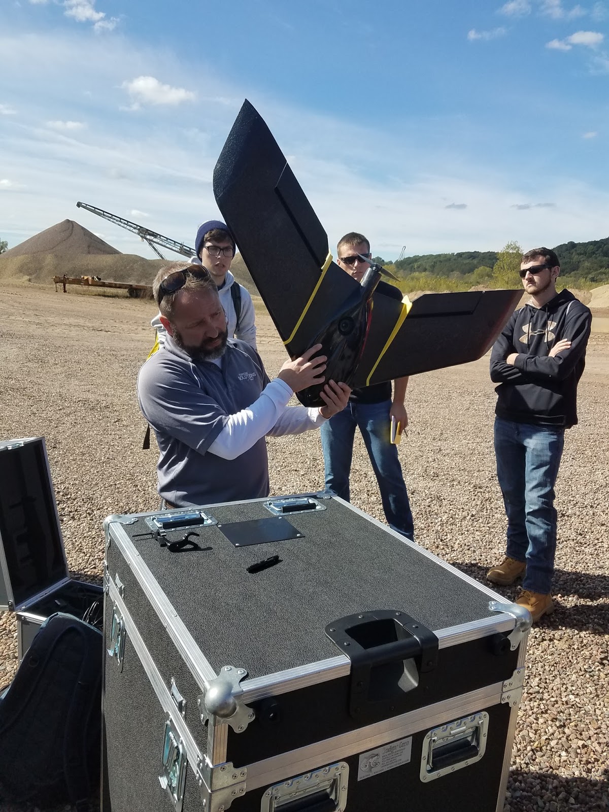
Figure 7: Here Josh from Topcon Solutions prepares the Ebee Plus for flight.  

Next Josh from TopCon Solutions flew the Ebee Plus.  This is a fixed wing aircraft with a mostly Styrofoam and plastic body.  It has a 20 megapixel camera, it is hand-launched and can be controlled from any PC.  Once launched, it hovers around "home" until you verbally command it to "go to mission".  This drone actually malfunctioned shortly, then after Josh commanded it to "come back to home" it encountered complete failure.  It flew off track and spiraled downward, crashing into the Chippewa River a couple hundred yards away.  Because it floated, it was able to be rescued down-river within an hour.  This was the first time Josh said he encountered this type of malfunction with the Ebee Plus.

Figure 8: Peter Menet flies the M600 Pro with Zenmuse X5.  This one is more expensive and powerful so the launching/landing area must be coned off.  

Figure 8 shows Peter Menet launching the M600 Pro with Zenmuse X5.  This is a multi-rotor drone with an external camera and has five battery packs.  The more battery packs it can hold, the longer the flight time ability.  This drone records RTK, which stands for Real Time Kinetics.

Figure 9: Peter Menet prepares the C-Astral Bramor w/ Sony a6000 for flight.  

The C-Astral Bramor w/ Sony a6000 is a fixed wing drone that has a launching stand.  The preparation for the flight was exhaustive in order to make sure it was launched correctly.  It is cranked tight with the large red rubber chords then launched into the air.  This drone also ended up crashing, which is very unusual to have two drones fail in the same day.  The parachute ended up not deploying and it crashed into a tree, completely destroying the body of the aircraft.

Figure 10: Josh Nave from Topcon Solutions shows how the Topcon Robotic Total Station is used to measure/model a gravel pile.  

Josh from Topcon also gave a demonstration of the Topcon Robotic Total Station, which can be used to survey an object or area with very high accuracy.  The station scans objects with a laser every three seconds.  It can do volumetrics, but the time it would take to scan the pile in the background was roughly an hour.  So it is very accurate, but very time consuming. 


Results

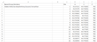
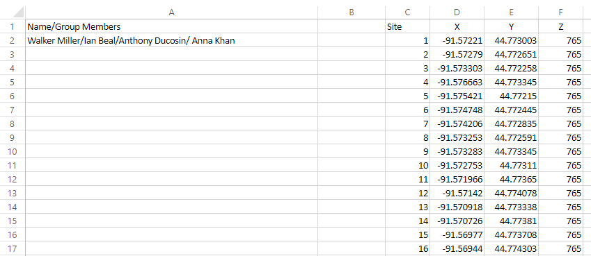
Figure : This is the excel spreadsheet that includes the data collected from the iphone for our group, with the z coordinate being the elevation unit.  

Conclusion
This fieldwork proved to be a valuable experience in learning about UAS platforms and surveying with this cutting edge technology.  The professionals from Topcon Solutions and Menet Aero were good resources in providing us with background information about each of their devices, as well as informing us about the surveying industry.  This technology may begin to become the main way in which volumetrics is modeled and measured in the surveying industry.

The fixed wing drones may be more expensive and seem more reliable than the rotary wing drones, but after observing the two fixed wing drones crash it seems that the rotary wing drones may be more reliable in similar conditions to what we had on Saturday.  It should also be noted that insurance for these drones is very important.  The total number of dollars in equipment used throughout the day was up to a couple hundred thousand dollars, so having insurance on this equipment is vital just in case accidents do happen.

We were able to conclude that the GPS in smart phones is much less accurate than the Bad Elf, and the data that will be processed later will probably reveal that it is far less accurate than the survey grade GPS devices.

Distance Azimuth Survey Method Activity

Introduction

This activity was conducted in order to learn how to conduct a survey using the concepts of distance and azimuth (direction).  These methods can be used to fall back on if other more advanced technology is not being reliable.  It works in many different circumstances and conditions and is quite simple, so knowing these methods could end up becoming useful in the field.

The objective of this activity was to work with a partner to collect spatial data in the field with a partner and create a map of the location and other attributes of the chosen trees.

Definitions:
Distance - the amount of space between two objects.

Azimuth - the horizontal angle or direction of a compass bearing.

Circumference - the girth or distance around an object.

Diameter - the distance of a straight line passing through the center of a circle to each side of the circle.

Methods

For this activity the two partners chose two sites along Putnam Drive on UW-Eau Claire's campus from which to locate, measure, and collect data about ten trees nearby.  The site map in Figure 1 shows the location of my group's two chosen sites.  The conditions of the day were sunny, humid, and warm, with most of Putnam Drive being shaded by the forest.

Figure 1: This site map shows the location of each site on UW-Eau Claire's lower campus along Putnam Drive.  

The tools used included: measuring tape, compass, GPS Pro device, distance laser, field notebook, and camera.  These items are shown in Figure 2.  The measuring tape was used to measure the circumference of the tree.  The compass was used to find the azimuth from the origin point to each chosen tree.  The GPS Pro device was used to mark the location of the origin.  The distance laser was used to measure the exact distance from the origin point to each chosen tree.  All the information collected was organized and recorded in the field notebook, and the camera took the pictures for the report.

Figure 2.01: The measuring tape was used to measure circumference of the trees.

Figure 2.02: The compass was used to find the azimuth.  

Figure 2.03: The GPS Pro unit was used to mark the point of origin.  

Figure 2.04: The distance laser was used to measure the exact distance from the point of origin to each tree.  

Site 1 was chosen by setting down the leather compass case and recording the coordinates of that spot with the GPS Pro.  This can be seen in Figure 3.  One student would stand directly above that spot and hold the distance laser to his/her chest and point the laser at the desired tree to get the distance to the tree.  That same person would stay in the same position and use the compass to find the azimuth from that spot to the same tree.  The other student would at the same time go to each tree and use the measuring tape to find the circumference of the tree and also try to determine the type/species of the tree if possible.  All this information was recorded in the field notebook.  This same method was used at Site 2.  One tip for recording trees is to go in order in one direction, say from left to right.  This way if any attributes are missed you can easily find which tree you need to remeasure or what have you.

Figure 3: Morgan is using the GPS Pro to find the location of the point of origin at Site 1.  

Once all the tree data was collected it was then manually put into an excel sheet, as shown in Figure 4.  The circumference was then used to find the diameter of each tree using a simple formula.  Also since the angles that the compass gave were divided into quadrants, each azimuth must be calculated into the corresponding angle within 360 degrees, with North being 0 degrees.

Figure 4: This image shows the excel sheet that was created to organize the data collected in the field.  

Next, a database was created using ArcCatalog as a place to import the data in the excel sheet as a table and to store all the results.  Each point was then brought onto the map by right clicking on the table in the table of contents, and setting the x field as longitude and the y field as the latitude.  The geographic coordinate system should be set as GCS_WGS_1984.  This can be seen in Figure 5.

Figure 5: This is the step to display the XY data as points on the map.  

Next the Feature Vertices To Points command was used to create a feature class containing the location of the trees as points.  The search bar was used to find this tool, as shown in Figure 6.  A basemap was also added to give context to the location of the points and the sites.

Figure 6: The Search bar was used to locate and use the Feature Vertices to Points tool. 

Then the Bearing Distance To Line command was used to connect the points of each tree to the origin point with a line, which was also found using the Search bar as seen in Figure 7.

Figure 7: The Search bar was used to locate and use the Bearing Distance to Line tool.  

Now that the data has been mapped it can be made into a more aesthetically pleasing map to be used to analyze the accuracy of the methods used in this activity.

Results

Figure 8 shows the final map created in ArcMap.

Figure 8: This is the final map result of the collected data in the field.  

This map shows that the point of origin for Site 1 was not accurate.  Each site has on the actual dirt road, and Site 1 in the map shows it being in the woods, off the road.  Site 2 seems to be accurate.

Because all the trees chosen in this activity were deciduous and the exact species of every tree was not known, the type was not specified in this map.

The distance and angle of each tree's azimuth in reference to the point of origin seems quite accurate however, and representing them by size was easy to display using ArcMap.

Conclusion

The azimuth distance survey methods incorporated in this activity were useful in locating features around a given point of origin.  The precision of the GPS unit will however affect the accuracy of the final product when brought into ArcMap.  These basic methods could be used in the field if the more advanced technology fails. 

Sandbox Activity

Introduction
The objective of this lab was to be introduced to sampling by using improvised surveying techniques.

Sampling definition: a shortcut method for investigating a whole population in which data is collected from a small portion of the population in order to get an idea of what the whole population is like.  Sampling from a spatial perspective means that data is collected in certain spots throughout a given area to get a better understanding of the area.  It can be done to create topographic maps, analyze population data, or observe various other types of information. 

Sampling techniques:
-Random: data is collected randomly.
-Systematic: data is collected systematically/evenly.
-Stratified: data is collected systematically, but data is collected more extensively in specified areas. 

Methods
Figure 1 shows the location of the sandbox site, on the eastern side of the Phillips science building on lower campus.  

Figure 1: This map shows the sandbox site location on UW - Eau Claire's lower campus.

The materials for this activity included: a sandbox (approx. 4ft x 4ft), tacs, string, a measuring stick, a field notebook, and a camera. 

Our group chose to use a stratified sampling technique.  We did this in order to get a more detailed survey of the area of interest.  It was a systematic approach, and we just decided to sample the central area of the sandbox with more data collection points.

Using the top of the sandbox border, we set up a grid system using the tacs and string, as seen in Figure 2.  The vertical strings were spaced every 5cm, as well as the horizontal strings in the central area of the sandbox in order to collect the most data points where the landscape had more features/variation. 

Figure 2: This image shows the strings being strung between the tacs that were distributed every 5cm on the top of the borders of the sandbox. 

Our "sea level" was at the level where the grid was strung across the top of the sandbox borders, so all of our measurements were measured in distance below "sea level". Using the measuring stick to measure at the intersection of each string as a point on the grid, each x/y coordinate was measured with a z record as elevation at that point.  This process is shown in Figure 3.

Figure 3: This image shows how the measuring stick was used to measure the distance from the "sea level" to the landscape floor at that specific point. 

One person acted at the measuring stick holder, another read each measurement aloud, and the third person recorded these measurements in a field notebook, which is shown in Figure 4.  This data would then be used later to create a digital elevation map. 

Figure 4: This image shows how each measurement was recorded into a field notebook. 

Results
Figure 5 displays the final result of this activity thus far.  Each point was entered manually into an excel spreadsheet. 

Figure 5: This image contains the final result of this activity at this time: all the measurements within an excel spreadsheet.

Once the group chose the sampling technique, that method did not change throughout the data collection process in order to not have inconsistent data.  This method worked quite well in collecting the data, and the resulting spreadsheet contains fairly consistent data.  One concern that was discovered was that the strings may not have been tight enough to remain perfectly level throughout the grid, so each string was re-tightened to account for this.  Other than that, the preparation for our data collection made the process quite smooth.  As the group proceeded, each member became faster and more efficient until all the measurements were collected.  Roles were even swapped in order to relieve each other of the more strenuous jobs. 

Conclusion
The sampling conducted in this activity was a good representation of the ways spatial sampling can be done on a much larger physical scale and with much larger data and more variables.  This sampling method allowed us to virtually map the sandbox quite accurately with just simple tools and the collection of a couple hundred data points.  This activity is just a small version of how data can be collected for a very large area.  When satellites or other aircraft capture images or lidar data of the Earth which are then used to analyze that area, they are also collecting specific information for specific points on the Earth as we did in the sandbox.  I believe our sampling did an adequate job in surveying the landscape within the sandbox.